41 how to display data labels above the columns in excel

How to Add Data Labels to an Excel 2010 Chart - dummies On the Chart Tools Layout tab, click Data Labels→More Data Label Options. The Format Data Labels dialog box appears. You can use the options on the Label Options, Number, Fill, Border Color, Border Styles, Shadow, Glow and Soft Edges, 3-D Format, and Alignment tabs to customize the appearance and position of the data labels. Text Labels on a Vertical Column Chart in Excel - Peltier Tech In the first table of this post (just below the first chart) you see three data columns: questions, ratings, and errors. Select the first two columns (including the top row with the blank cell and the "Response" label) and make your chart, and it will automatically use those labels for the category axis labels.

Using Microsoft® Excel to Plot and Analyze Kinetic Data • Adjust column widths to fit the labels by clicking on the column heading and dragging the border to the appropriate width Enter your data pairs in the appropriate columns. (Don’t forget to enter 0,0 for one of your data pairs.) If your data was not collected in order of increasing substrate concentration, enter the data pairs in the order ...

How to display data labels above the columns in excel

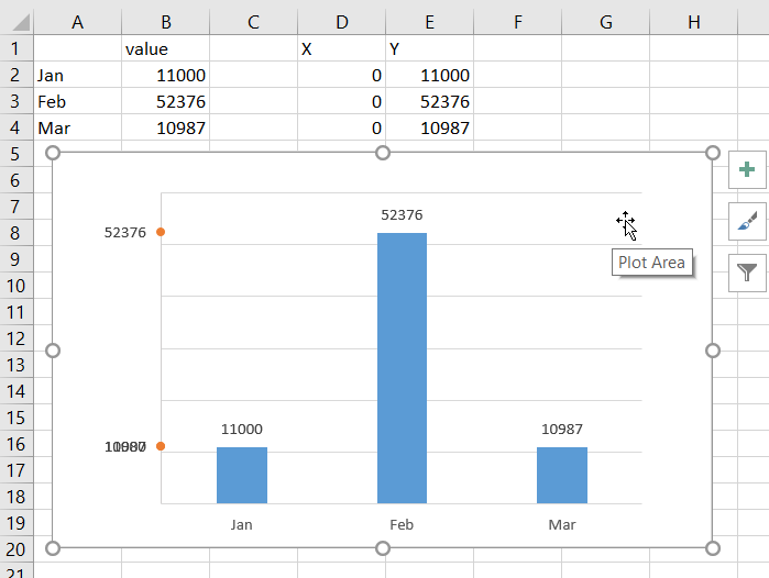
data visualization - How do you put values over a simple ... 1) Select cells A2:B5 2) Select "Insert" 3) Select the desired "Column" type graph 4) Click on the graph to make sure it is selected, then select "Layout" 5) Select "Data Labels" ("Outside End" was selected below.) Format Data Labels in Excel- Instructions - TeachUcomp, Inc. One way to do this is to click the "Format" tab within the "Chart Tools" contextual tab in the Ribbon. Then select the data labels to format from the "Current Selection" button group. Then click the "Format Selection" button that appears below the drop-down menu in the same area. 5 Ways to Concatenate Data with a Line Break in Excel May 02, 2022 · Paste the above formula into the formula bar and press Enter to confirm the new step. This formula will create a new column in the data where each row is the result of concatenating the data from the other columns with the power query line break character #(lf). Now we can Close and Load the data from the Home tab.

How to display data labels above the columns in excel. Data Labels above bar chart - Excel Help Forum For a new thread (1st post), scroll to Manage Attachments, otherwise scroll down to GO ADVANCED, click, and then scroll down to MANAGE ATTACHMENTS and click again. Now follow the instructions at the top of that screen. New Notice for experts and gurus: Excel tutorial: How to use data labels When first enabled, data labels will show only values, but the Label Options area in the format task pane offers many other settings. You can set data labels to show the category name, the series name, and even values from cells. In this case for example, I can display comments from column E using the "value from cells" option. Leader lines ... Column Chart That Displays Percentage ... - Excel Campus Create the Column Chart. The first step is to create the column chart: Select the data in columns C:E, including the header row. On the Insert tab choose the Clustered Column Chart from the Column or Bar Chart drop-down. The chart will be inserted on the sheet and should look like the following screenshot. 3. How to Create a Bar Chart With Labels Above Bars in Excel In the Format Data Labels pane, under Label Options selected, set the Label Position to Inside Base. 10. Then, under Label Contains, check the Category Name option and uncheck the Value and Show Leader Lines options. 11. Next, while the labels are still selected, click on Text Options, and then click on the Textbox icon. 12.

How to Add Total Data Labels to the Excel Stacked Bar ... For stacked bar charts, Excel 2010 allows you to add data labels only to the individual components of the stacked bar chart. The basic chart function does not allow you to add a total data label that accounts for the sum of the individual components. Fortunately, creating these labels manually is a fairly simply process. Solved: Matrix - Display Values above Columns - Microsoft ... If you want to display data like the format in Tableau, you need to unpivot Value and SpreadCost columns. Please right click your table->Query Editor->select both Value and SpreadCost columns->Unpivot columns (see the button highlighted in yellow background), click apply, you will get the data shown in screenshot. Create Dynamic Chart Data Labels with Slicers - Excel Campus You basically need to select a label series, then press the Value from Cells button in the Format Data Labels menu. Then select the range that contains the metrics for that series. Click to Enlarge Repeat this step for each series in the chart. If you are using Excel 2010 or earlier the chart will look like the following when you open the file. Add or remove data labels in a chart Right-click the data series or data label to display more data for, and then click Format Data Labels. Click Label Options and under Label Contains, select the Values From Cells checkbox. When the Data Label Range dialog box appears, go back to the spreadsheet and select the range for which you want the cell values to display as data labels.

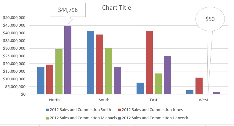
Tutorial: Import Data into Excel, and Create a Data Model In the next tutorial, Extend Data Model relationships using Excel 2013, Power Pivot, and DAX, you build on what you learned here, and step through extending the Data Model using a powerful and visual Excel add-in called Power Pivot. You also learn how to calculate columns in a table, and use that calculated column so that an otherwise unrelated ... Add a Data Callout Label to Charts in Excel 2013 ... In the upper right corner, next to your chart, click the Chart Elements button (plus sign), and then click Data Labels. A right pointing arrow will appear, click on this arrow to view the submenu. Select Data Callout. Once the Data Callout Labels have been added, you can re-position them by clicking on their borders and dragging to a new position. Text Labels on a Horizontal Bar Chart in Excel - Peltier Tech Dec 21, 2010 · In this tutorial I’ll show how to use a combination bar-column chart, in which the bars show the survey results and the columns provide the text labels for the horizontal axis. The steps are essentially the same in Excel 2007 and in Excel 2003. I’ll show the charts from Excel 2007, and the different dialogs for both where applicable. Quick Tip: Excel 2013 offers flexible data labels ... With the cursor inside that data label, right-click and choose Insert Data Label Field. In the next dialog, select [Cell] Choose Cell. When Excel displays the source dialog, click the cell that...

November 2018

charts - Excel, giving data labels to only the top/bottom ... 1) Create a data set next to your original series column with only the values you want labels for (again, this can be formula driven to only select the top / bottom n values). See column D below. 2) Add this data series to the chart and show the data labels. 3) Set the line color to No Line, so that it does not appear! 4) Volia! See Below! Share

Is it possible to display the exact value on the y-axis on a - Microsoft Community

How to add live total labels to graphs and charts in Excel ... Step 3: Format your totals. Now all the totals are represented on a line. To make it appear as if these totals are just connected to the top of each column, first select the line and change the colour to No outline.Then select all the total labels and right click to select Format Data Label.Change the label position to Above.You can follow the same steps in both Excel and PowerPoint.

Quick Tip: Excel 2013 offers flexible data labels - TechRepublic

Guide: How to Name Column in Excel | Indeed.com Choose the "Advanced" option in the left navigation pane to the Display options for this worksheet section. Uncheck the box for "Show row and column headers." When you return to the worksheet, the column title row is the only column header that would be visible. To make the default column header re-appear, you can re-check the box. 2.

Display the data labels on this chart above the data markers

How to add total labels to stacked column chart in Excel? Select the source data, and click Insert > Insert Column or Bar Chart > Stacked Column. 2. Select the stacked column chart, and click Kutools > Charts > Chart Tools > Add Sum Labels to Chart. Then all total labels are added to every data point in the stacked column chart immediately. Create a stacked column chart with total labels in Excel

PPC Storytelling: How to Make an Excel Bubble Chart for PPC

How to Show Percentages in Stacked Column Chart in Excel ... Step 3: To create a column chart in excel for your data table. Go to "Insert" >> "Column or Bar Chart" >> Select Stacked Column Chart . Step 4: Add Data labels to the chart. Goto "Chart Design" >> "Add Chart Element" >> "Data Labels" >> "Center". You can see all your chart data are in Columns stacked bar.

Which Excel chart should I use to display this complex data? - Quora

How to add data labels from different column in an Excel ... Click any data label to select all data labels, and then click the specified data label to select it only in the chart. 3. Go to the formula bar, type =, select the corresponding cell in the different column, and press the Enter key. See screenshot: 4. Repeat the above 2 - 3 steps to add data labels from the different column for other data points.

How-to Use Data Labels from a Range in an Excel Chart - Excel Dashboard Templates

Pivot table - Wikipedia There will also be one added column of Total. In the example above, this instruction will create five columns in the table — one for each salesperson, and Grand Total. There will be a filter above the data — column labels — from which one can select or deselect a particular salesperson for the pivot table.

Stop Excel Overlapping Columns on Second Axis for 3 Series

Display Missing Dates in Excel PivotTables • My Online ... Mar 25, 2014 · Note: Apply 'Wrap Text' format to column B of your Table if you want to see your date text string formatted as per the image above, i.e. with the date number above the letter for the day. However, this is not necessary for the PivotChart since it wraps the text because we have used the CHAR(10) character in the text string.

Share :