43 pivot table excel row labels side by side

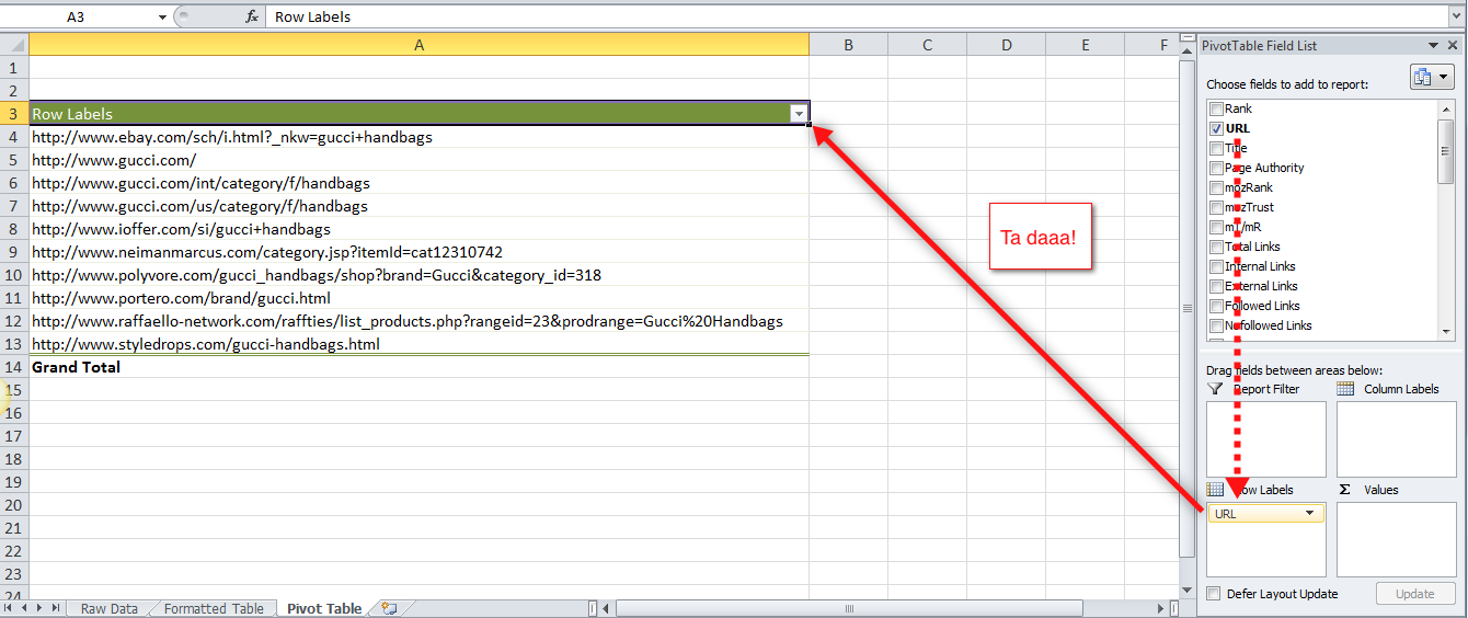
Pivot Table Row Labels In the Same Line - Beat Excel! First make a pivot table with required fields. Arrange the fields as shown in left picture. Your initial table will look like right picture. Now click on "Error Code" and access field settings. First check "None" option in "Subtotals & Filters" tab to disable totals after every row. Pivot table row labels side by side - Excel Tutorials You can copy the following table and paste it into your worksheet as Match Destination Formatting. Now, let's create a pivot table ( Insert >> Tables >> Pivot Table) and check all the values in Pivot Table Fields. Fields should look like this. Right-click inside a pivot table and choose PivotTable Options…. Check data as shown on the image below.

Repeat first layer column headers in Excel Pivot Table Right-click the row or column label you want to repeat, and click Field Settings. Click the Layout & Print tab, and check the Repeat item labels box. Make sure Show item labels in tabular form is selected. Tested just now and it worked for column headers. Thanks for the link, Alan.

Pivot table excel row labels side by side

How to Flatten and repeat Row Labels in a Pivot Table - YouTube Excelerator BI 4.5K subscribers Subscribe This video shows you how to easily flatten out a Pivot Table and make the row labels repeat. This is useful if you need to export your data and share it... How to make row labels on same line in pivot table in excel #ExcelMaster, #PivotTable, #ExcelHow to make row labels on same line in pivot table in excelHow to show multiple rows in pivot table in excel How to repeat row labels for group in pivot table? - ExtendOffice In Excel, when you create a pivot table, the row labels are displayed as a compact layout, all the headings are listed in one column. Sometimes, you need to convert the compact layout to outline form to make the table more clearly. But in tphe outline layout, the headings will be displayed at the top of the group.

Pivot table excel row labels side by side. Design the layout and format of a PivotTable In the PivotTable, right-click the row or column label or the item in a label, point to Move, and then use one of the commands on the Move menu to move the item to another location. Select the row or column label item that you want to move, and then point to the bottom border of the cell. Excel Pivot Table with nested rows - Basic Excel Tutorial Table of Contents. Steps. How to add the fields. Nested Pivot Table. 1. Insert your pivot table. Click Insert Menu, under Tables group choose PivotTable. 2. Once you create your pivot table, add all the fields you need to analyze data. How to make row labels on same line in pivot table? Make row labels on same line with PivotTable Options You can also go to the PivotTable Options dialog box to set an option to finish this operation. 1. Click any one cell in the pivot table, and right click to choose PivotTable Options, see screenshot: 2. How to Use Excel Pivot Table Label Filters Watch the steps in this short video, and the written instructions are below the video. Play. To change the Pivot Table option to allow multiple filters: Right-click a cell in the pivot table, and click PivotTable Options. Click the Totals & Filters tab Under Filters, add a check mark to 'Allow multiple filters per field.'.

Combining row labels in pivot table : excel - reddit Okay so I'm using a pivot table and i have the column I want as the row labels. The problem is some of the data represents the same thing but aren't identical so they get different rows. As an example if the row labels are salesman and some of the cells from the raw table have James Bond and others have bond, or JB. Multiple row labels on one row in Pivot table - MrExcel I figured it out - Right click on your pivot table and choose pivot table options/display. Click on "Classic PivotTable layout" Then click on where it is subtotaling your row label and uncheck the subtotal option. D dudeshane0 New Member Joined Oct 23, 2014 Messages 1 Jan 19, 2015 #6 Gerald Higgins said: Pivot Table column label from horizontal to vertical Pivot Table column label from horizontal to vertical After pivot table and with grouping, some column labels have been showed but the caption is on the top. What i want is put the column header at the left of the row as vertical red text show as below. However, i cannot do this, it said "We cant change this part of pivot table". Excel 2007 Pivot Table side by side row labels [SOLVED] Excel 2007 Pivot Table side by side row labels Hi Masters In Excel 2003 I could add 2 data elements to the Row label area of the Pivot table. Both items would show up on each row in a different column, this does not happen in 2007 as all items in the row label show up in the same column. How can I revert to the way it was in 2003? Many thanks

Excel tutorial: How to filter a pivot table by rows or columns When you add a field as a row or column label in a pivot table, you automatically get the ability to filter the results in the table by items that appear in that field. Let's take a look. This pivot table is displaying just one field: Total Sales. After we add Product as a row label, notice that a drop-down arrow appears in the header area. How to Customize Your Excel Pivot Chart Data Labels - dummies The Data Labels command on the Design tab's Add Chart Element menu in Excel allows you to label data markers with values from your pivot table. When you click the command button, Excel displays a menu with commands corresponding to locations for the data labels: None, Center, Left, Right, Above, and Below. Automatic Row And Column Pivot Table Labels - How To Excel At Excel Select the data set you want to use for your table The first thing to do is put your cursor somewhere in your data list Select the Insert Tab Hit Pivot Table icon Next select Pivot Table option Select a table or range option Select to put your Table on a New Worksheet or on the current one, for this tutorial select the first option Click Ok How to add side by side rows in excel pivot table - AnswerTabs To display more pivot table rows side by side, you need to turn on the Classic PivotTable layout and modify Field settings. For example will be used the following table: You have to right-click on pivot table and choose the PivotTable options. Then swich to Display tab and turn on Classic PivotTable layout:

Pivot table row labels side by side – Excel Tutorials

07 Pivot Table side by side row labels - groups.google.com - Go to PivotTable Tools, then Options - in the Active Field, select Field Settings - In the Field Settings box, select the 2nd tab 'Layout & Print' - Under 'Show item labels in outline form',...

31 How To Label Excel Columns - Labels Database 2020

Repeat item labels in a PivotTable - support.microsoft.com Right-click the row or column label you want to repeat, and click Field Settings. Click the Layout & Print tab, and check the Repeat item labels box. Make sure Show item labels in tabular form is selected. Notes: When you edit any of the repeated labels, the changes you make are applied to all other cells with the same label.

Download Advanced Pivot Table Excel 2010 | Gantt Chart Excel Template

Pivot Table Row Labels • AuditExcel.co.za How to work with Pivot Table row labels in Excel 2007 and up. For updated video clips in structured Excel courses with practical example files, have a look at our MS Excel online training courses . You can even try the Free MS Excel tips and tricks course.; To see if this video matches your skill level (see the suggested skill score below) do our free MS Excel skills assessment.

How To Manage Big Data With Pivot Tables

Pivot table row labels in separate columns • AuditExcel.co.za Our preference is rather that the pivot tables are shown in tabular form (all columns separated and next to each other). You can do this by changing the report format. So when you click in the Pivot Table and click on the DESIGN tab one of the options is the Report Layout. Click on this and change it to Tabular form.

Pivot table row labels in separate columns • AuditExcel.co.za

How to Add Rows to a Pivot Table: 9 Steps (with Pictures) 3. Drag a field into the "Rows" area on PivotTable Fields. When you drag any of the fields in the upper portion of the PivotTable Fields panel to Rows, a new row will be added to your table. Rows are usually non-numeric fields, such as column headers. Numbers will usually go into the Values area. [1]

Pivot Table in Excel - A Beginners Guide for Excel Users

Multi-level Pivot Table in Excel (In Easy Steps) First, insert a pivot table. Next, drag the following fields to the different areas. 1. Country field to the Rows area. 2. Amount field to the Values area (2x). Note: if you drag the Amount field to the Values area for the second time, Excel also populates the Columns area. Pivot table: 3. Next, click any cell inside the Sum of Amount2 column. 4.

Putting Data into a Pivot Table Report - Excel 2007 VBA

columns side by side in pivot table - Microsoft Community Drag first name and last name in Rows area and turn off total, if needed Design tab > Report Layout > Show in Tabular form Sincerely yours, Vijay A. Verma @ Report abuse 10 people found this reply helpful · Was this reply helpful?

How to Save Time and Energy with Pivot Tables in Microsoft Excel | Depict Data Studio

How to repeat row labels for group in pivot table? - ExtendOffice In Excel, when you create a pivot table, the row labels are displayed as a compact layout, all the headings are listed in one column. Sometimes, you need to convert the compact layout to outline form to make the table more clearly. But in tphe outline layout, the headings will be displayed at the top of the group.

Share :