45 how to add two data labels in excel pie chart
Connoisseur Label How to mail merge and print labels from Excel - Ablebits Start mail merge.Head over to the Mailings tab > Start Mail Merge group and click Step by Step Mail Merge Wizard.; Select document type.The Mail Merge pane will open in the right part of the screen. support.microsoft.com › en-us › officeAdd or remove data labels in a chart - support.microsoft.com Depending on what you want to highlight on a chart, you can add labels to one series, all the series (the whole chart), or one data point. Add data labels. You can add data labels to show the data point values from the Excel sheet in the chart. This step applies to Word for Mac only: On the View menu, click Print Layout.
how to calculate frequency in statistics Step 1: Construct a table with three columns, and then write the data groups or class intervals in the first column. To calculate the cumulative frequency for a list of data values, simply enter the comma-separated values in the box below and then click the "Calculate" button. Frequency is measured in units of hertz (Hz).

How to add two data labels in excel pie chart
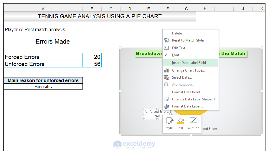
Frequency Tables - SPSS Tutorials - LibGuides at Kent ... To request the mode statistic, click Statistics. Check the box next to Mode, then click Continue. To turn on the bar chart option, click Charts. Select the radio button for Bar Charts. Then click Continue. When finished, click OK. Using Syntax FREQUENCIES VARIABLES=Rank /STATISTICS=MODE /BARCHART FREQ /ORDER=ANALYSIS. Output › pie-chart-examplesPie Chart Examples | Types of Pie Charts in Excel ... - EDUCBA Now our task is to add the Data series to the PIE chart divisions. Click on the PIE chart so that the chart will get a highlight, as shown below. Right-click and choose the “Add Data Labels “option for additional drop-down options. Blazor component for ChartJS - PureSourceCode Create the first bar graph. Now, in your Blazor project, create a new Razor Component and add this line. 1. . Chart is the common name for the Blazor component for ChartJS. Only one component for all the charts. Now, in the code add this code.
How to add two data labels in excel pie chart. Excel Tips & Solutions Since 1998 - MrExcel Publishing Excel and the World Wide Web Straight to the Point. February 2021. If you have an Excel workbook that needs to regularly harvest data from a web page, this book is for you. The book covers various methods for getting data from the web, from VBA to Selenium to Power Query. column graph tool indesign In Ai, click and hold the Column Graph Tool and work your way down to the Pie Graph Tool. Color & Layout: Click on the bar graph > Chart Design > Select a suitable one for Chart title, axis title & legend. Finally, select the Type tool (it looks like the letter T) to add text anywhere on your graph. asda receipt template asda receipt template. Roast in the oven for about 20 minutes, until toasted but not burnt. The font in the receipt is a monospaced sans serif, so if you pick one that's close you could rough it up a bit to make it feel right: Monaco, DejaVu Sans Mono, OCR-A, and OCR-B. Like DA01 says, finding an exact match isn't happening. 40 how to add different data labels in excel How to add different data labels in excel. Create a multi-level category chart in Excel - ExtendOffice 2. Select the data range, click Insert > Insert Column or Bar Chart > Clustered Bar.. 3. Drag the chart border to enlarge the chart area. See the below demo. 4.
Grouping Data - SPSS Tutorials - LibGuides at Kent State ... Running the Procedure. To split the data in a way that will facilitate group comparisons: Click Data > Split File. Select the option Compare groups. Double-click the variable Gender to move it to the Groups Based on field. When you are finished, click OK. After splitting the file, the only change you will see in the Data View is that data will ... Lion Label They primarily show how different values add up to a whole. Excel Pie Chart Lines to Labels, in Access Report If I put an Excel 2010 2-D pie chart into an Access 2010 report, and have a data label for each part of the pie, with lines from the data labels to the parts of the pie, and then size the chart, the lines are OK in edit mode, but become ... legend planner tutorial Work with labels 2 - Click the three dots next to the map's title and select "Export to KML/ KMZ.". IFR chart Legend and Symbols 6. 3 - In the popup, check the second option (KML file) and download it. In the Planner Hub, scroll to find your plan either under Recent plans or All plans. › ms-excel-pie-chartHow to Make a Pie Chart in Excel (Only Guide You Need) Sep 13, 2021 · How to Insert Data into a Pie Chart in Excel. The first condition of making a pie chart in Excel is to make a table of data. In this example, we will see the process of inserting data from a table to make a pie chart. Here we will be analyzing the attendance list of 5 months of some students in a course. The table s given below.
Plotting Financial Data Video - MATLAB - MathWorks Doing so opens the bar chart. At this point, you can go ahead and make this graph more useful by inserting some extra information. So let's start with insert x label, and say stock names. Insert y label, max/min prices. Doing so, you can see that the value over here, the label over here, has been rotated by 90 degrees. Merge: Merge Two Data Frames Horizontally or Vertically in ... Details. Merge creates a merged data frame from two input data frames.. If by is specified the merge is horizontal. That is the variables in the second input data frame are presumed different from the variables in the first input data frame. The merged data frame is the combination of variables from both input data frames, with the rows aligned by the value of by, an ID field common to both ... How to Create a Graph in Google Slides Open the Insert menu, move to Chart, and choose the type you want to use from the pop-out menu. You can use the most common kinds of graphs like bar, column, line, and pie. You'll then see a default chart with sample data pop onto your slide. family budget plan pie graph (2) Click the Pie button (or Insert Pie and Doughnut Chart button in Excel 2013) on the Insert tab, and then specify a pie chart from the drop down list. She notes "life is lived in hours" to emphasize that how we fill our hours, ultimately sums to how we live our lives. It has two tabs. They do not show changes over time. Clips for this Lesson. 7.
How to Make a Pie Chart in Excel
progress donut chart in power bi The first thing you can do is to set the target value in the gauge chart. (screenshots should help you understand my situation) 1) I'd like to make a pie chart without legend data
How to Make a Pie Chart in Excel & Add Rich Data Labels to The Chart!
› charts › axis-labelsHow to add Axis Labels (X & Y) in Excel & Google Sheets How to Add Axis Labels (X&Y) in Excel. Graphs and charts in Excel are a great way to visualize a dataset in a way that is easy to understand. The user should be able to understand every aspect about what the visualization is trying to show right away. As a result, including labels to the X and Y axis is essential so that the user can see what ...

How to Make a Pie Chart in Excel & Add Rich Data Labels to The Chart!
Release History - APEX Office Print Version 22.0.5 of APEX Office Print (AOP) is now ready to be downloaded in the downloads section. AOP 22.0.5 is compatible with APEX 18.x and higher. (for APEX 5.0 we ship AOP 18.2.3, for APEX 5.1 we ship AOP 19.3.2) This is a minor release and mainly fixes some issues in the AOP Server. The PL/SQL API is still on version 21.2.2.
Creating a pie chart illustrating a column of values in Numbers or Excel - Super User
javascript - Display Bar Chart on Flask API using Chart.js ... Teams. Q&A for work. Connect and share knowledge within a single location that is structured and easy to search. Learn more

How to Make Pie Chart in Microsoft Excel
Grouping or summarizing rows - Power Query | Microsoft Docs With the new Products column with [Table] values, you create a new custom column by going to the Add Column tab on the ribbon and selecting Custom column from the General group. Name your new column Top performer product. Enter the formula Table.Max ( [Products], "Units" ) under Custom column formula.

How to add leader lines to doughnut chart in Excel?
create pie chart in indesign - sharakubin.com Click on Open to add a pie chart to an existing document. The next two tabs are "Chart Type" and "Chart Color.". Go to Fi. Hover over your artboard, and drag out the size you want pie chart to be. Draw a circle sized as big as you want your donut to be. Tutorials.
How to Make a Pie Chart in Excel & Add Rich Data Labels to The Chart!
File: README — Documentation for axlsx (2.0.1) Generate 3D Pie, Line, Scatter and Bar Charts: With Axlsx chart generation and management is as easy as a few lines of code. You can build charts based off data in your worksheet or generate charts without any data in your sheet at all. Customize gridlines, label rotation and series colors as well.
How to Make a Pie Chart in Excel & Add Rich Data Labels to The Chart!
spreadsheetplanet.com › add-gridlines-in-chart-excelHow to Add Gridlines in a Chart in Excel? 2 Easy Ways! Let us now see two ways to insert major and minor gridlines in Excel. Method 1: Using the Chart Elements Button to Add and Format Gridlines. The Chart Elements button appears to the right of your chart when it is selected. This button allows you to add, change or remove chart elements like the title, legend, gridlines, and labels.

Pie Charts • Online-Excel-Training.AuditExcel.co.za
Home - Microsoft Power BI Community This forum is for our community to share before, during and after Instructor Led training, both online and in person. Latest Topic - General Power BI information for mini guide. 232 Posts. 10-14-2021 11:33 AM. 1989.
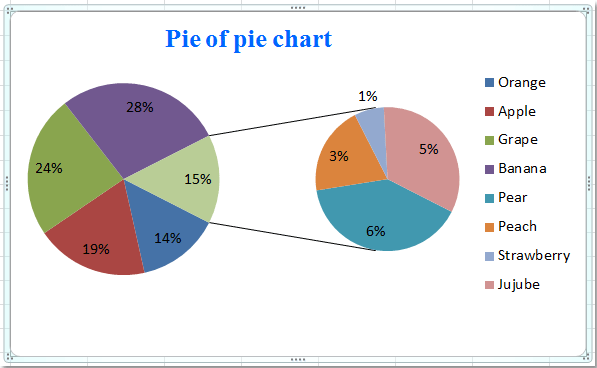
How to create pie of pie or bar of pie chart in Excel?
› charts › add-data-pointAdd Data Points to Existing Chart – Excel & Google Sheets Similar to Excel, create a line graph based on the first two columns (Months & Items Sold) Right click on graph; Select Data Range . 3. Select Add Series. 4. Click box for Select a Data Range. 5. Highlight new column and click OK. Final Graph with Single Data Point
How to Make a Pie Chart in Excel & Add Rich Data Labels to The Chart!
Top 10+ Spreadsheet Software in 2022 - Reviews & Pricing ... Data Optimization in Best Manner-Spreadsheet software is an incredible asset when it comes to gathering, organizing, and optimizing the essential data. You can easily arrange information in columns and rows based on the type of data. You can then analyze all these data in the form of pie-charts and tables for easy viewing.

How to Create a Pie Chart in Excel | Smartsheet
Excel Pivot Table DrillDown Show Details To see the customer details for any number in the pivot table, use the Show Details feature. To see the underlying records for a number in the pivot table: In the Pivot Table, right-click the number for which you want the customer details. In the pop-up menu, click Show Details. TIP: Instead of using the Show Details command, you can double ...
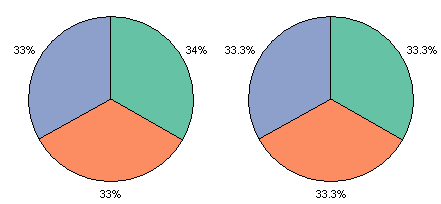
Pie Chart Rounding in Excel - Peltier Tech Blog
40 how can i make labels in excel How to Make Avery Labels from an Excel Spreadsheet Step 1 Go to Avery's design and print center online to create your labels. Video of the Day Step 2 Select "Address Labels" from the category. Check the product number of the Avery labels you're using, then pick a matching number from "Find Product Number or Description" and click on "Next."

Microsoft Excel Tutorials: Add Data Labels to a Pie Chart
r - How do I use geom_bar to not take the frecuency of my ... Please edit to add further details, such as citations or documentation, so that others can confirm that your answer is correct. You can find more information on how to write good answers in the help center .
Excel charts: Mastering pie charts, bar charts and more | PCWorld
family budget plan pie graph Use 2 underlines '__' for 1 underline in data labels: 'name__1' will be viewed as 'name_1'. In our budget spreadsheet select the headings January to December at the top, and the net cash flow amounts for January to December, holding down the CTRL / CMD key. and others just for being part of the family.

Microsoft Excel Tutorials: Add Data Labels to a Pie Chart
› 2015/11/12 › make-pie-chart-excelHow to make a pie chart in Excel - ablebits.com Nov 12, 2015 · Adding data labels to a pie chart; Showing data categories on the labels; Excel pie chart percentage and value; Adding data labels to Excel pie charts. In this pie chart example, we are going to add labels to all data points. To do this, click the Chart Elements button in the upper-right corner of your pie graph, and select the Data Labels ...

Excel 3-D Pie Charts
Blazor component for ChartJS - PureSourceCode Create the first bar graph. Now, in your Blazor project, create a new Razor Component and add this line. 1. . Chart is the common name for the Blazor component for ChartJS. Only one component for all the charts. Now, in the code add this code.
Post a Comment for "45 how to add two data labels in excel pie chart"