44 pivot table 2 row labels

Pivot table row labels side by side - Excel Tutorials Now, let's create a pivot table ( Insert >> Tables >> Pivot Table) and check all the values in ... Apply Multiple Filters on a Pivot Field - Excel Pivot Tables Right-click any cell in the pivot table, and click PivotTable Options. Click the Totals & Filters tab. Under Filters, add a check mark to 'Allow multiple filters per field.'. Click OK. Now you can apply both a Label filter and a Value filter to the OrderMth field, and both will be retained. In the screen shot below, both the Label filter ...

Design the layout and format of a PivotTable Click anywhere in the PivotTable. This displays the PivotTable Tools tab on the ribbon. On the Options tab, in the PivotTable group, click Options. In the PivotTable Options dialog box, click the Layout & Format tab, and then under Layout, select or clear the Merge and center cells with labels check box.

Pivot table 2 row labels

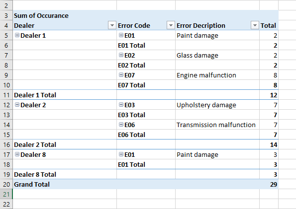
Pivot Table Row Labels In the Same Line - Beat Excel! Then navigate to "Layout & Print" tab and click on "Show item in tabular form" option. Do this procedure also for "Dealer" field and your table will look like this: If you also want dealer names to repeat on each row, reopen "Dealer field settings and check "Repear item labels" option in "Layout & Print" tab. Excel Pivot Table Row labels - Stack Overflow Right click on the pivot, go to PivotTable Options, Display Tab. Click on "Classic Pivot Table Layout" Go to each field (column), right click, field settings, layout & print tab. Click on "Repeat Item Labels" That should give you the table you're looking for. Share answered Nov 9, 2015 at 13:20 user1923975 1,359 3 13 28 Add a comment get a row label from pivot table - Microsoft Tech Community Hi all! I have a pivot table and I would like to get some information. For Example the green sqare. ... So the question is how to get a row label from pivot table in a cel that is not a pivot table . 0 Likes . Reply. Hans Vogelaar . replied to omdl2020 ‎Nov 13 2020 12:30 PM. Mark as New; Bookmark; Subscribe;

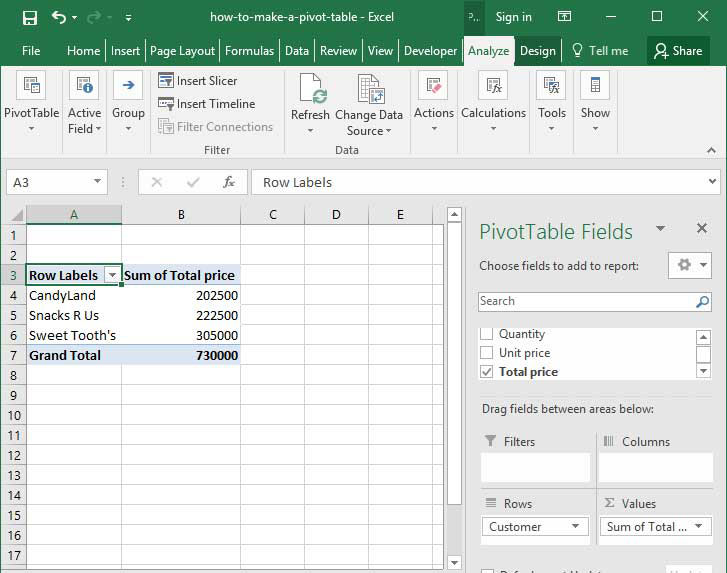
Pivot table 2 row labels. How to rename group or row labels in Excel PivotTable? 1. Click at the PivotTable, then click Analyze tab and go to the Active Field textbox. 2. Now in the Active Field textbox, the active field name is displayed, you can change it in the textbox. You can change other Row Labels name by clicking the relative fields in the PivotTable, then rename it in the Active Field textbox. How to Add Two-Tier Row Labels to the Pivot Table in Google Sheets Here are the steps to add the second-tier row label as the second column in the Pivot Table: Step 1: Click on any cell in the Pivot Table so that the Pivot table editor sidebar appears on the right side of Google Sheets. Pivot Table, with Pivot table editor sidebar visible. ‍. How to make row labels on same line in pivot table? 1. Click any one cell in the pivot table, and right click to choose PivotTable Options, see screenshot: 2. In the PivotTable Options dialog box, click the Display tab, and then check Classic PivotTable layout (enables... 3. Then click OK to close this dialog, and you will get the following pivot ... Ranking to a Pivot Table with multiple Row Labels I have a pivot table with multiple Row Labels: Team and Player. I created a second Pts column and used 'Show Values As - Rank Largest to Smallest', but it's not working. It's showing up as '1' for all columns, regardless of whether or not I pick 'Team' or 'Player' as the base field. If I remove 'Team' as a Row Label, however, it works perfectly.

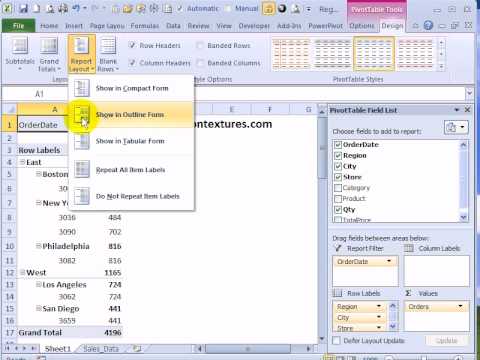
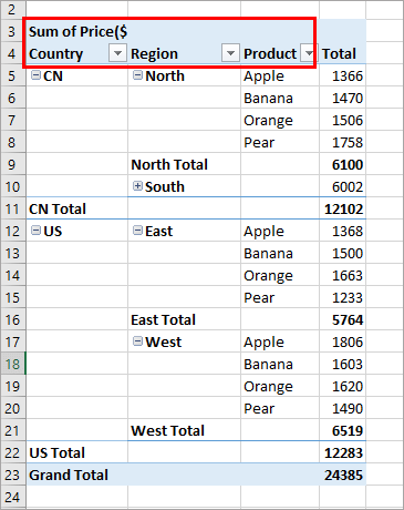
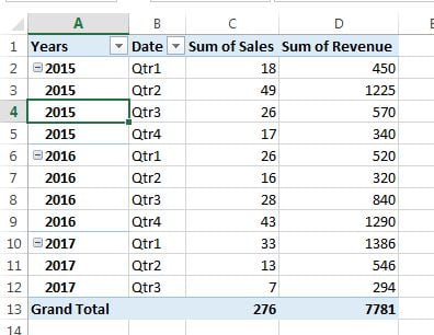
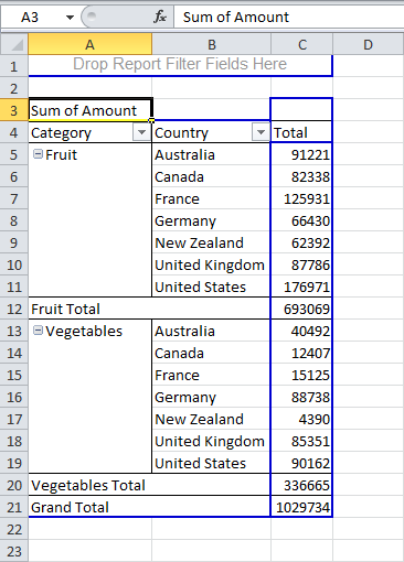
Pivot Table Multiple Row Labels? [SOLVED] You can, of course, create a pivot table that sums the values just at the owner level. then, create a second pivot table that sums the values at the Engineer level. If you need to present this data in a contiguous table, you can create a new Excel table and reference to the pivot table values with formulas (=PivotTableSheet!A1) cheers Microsoft MVP How to add side by side rows in excel pivot table - AnswerTabs First, you have to create a pivot table by choosing the rows, columns and values: Created pivot table should look like this: You have to right-click on pivot table and choose the PivotTable options. Then swich to Display tab and turn on Classic PivotTable layout: Now the pivot table should look like this: As a next step, you have to modify the Field settings of the rows: In subtotals section choose None: Pivot table row labels in separate columns • AuditExcel.co.za So when you click in the Pivot Table and click on the DESIGN tab one of the options is the Report Layout. Click on this and change it to Tabular form. Your pivot table report will now look like the bottom picture and will be easier to use in other areas of the spreadsheet and in our opinion is also easier to read. Multi-level Pivot Table in Excel - Easy Excel Tutorial First, insert a pivot table. Next, drag the following fields to the different areas. 1. Category field and Country field to the Rows area. 2. Amount field to the Values area. Below you can find the multi-level pivot table. Multiple Value Fields First, insert a pivot table. Next, drag the following fields to the different areas. 1.

How to Use Excel Pivot Table Label Filters To change the Pivot Table option, and allow multiple filters, follow these steps: Right-click a cell in the pivot table, and click PivotTable Options. In the PivotTable Options dialog box, click the Totals & Filters tab In the Filters section, add a check mark to 'Allow multiple filters per field.' python - how to repeat row labels in pandas pivot table function and ... April May Count Ratio Count Ratio Country Cities USA LA 2 1:2 3 4:5 USA FL 5 5:6 6 4:5 USA TX 7 1:3 2 1:4 Canada Ontario 2 1:3 6 8:9 Canada Toronto 3 1:5 9 3:4 I've tried pd.option_context('display.multi_sparse', False) , as it only display the content, it does not export data as excel. Multiple row labels on one row in Pivot table | MrExcel Message Board I figured it out - Right click on your pivot table and choose pivot table options/display. Click on "Classic PivotTable layout" Then click on where it is subtotaling your row label and uncheck the subtotal option. D dudeshane0 New Member Joined Oct 23, 2014 Messages 1 Jan 19, 2015 #6 Gerald Higgins said: How to repeat row labels in a pivot table - Ask LibreOffice Right click anywhere within pivot table. Select Edit Layout. Double click on Year (in my case) from Row Fields list. Data Field popup will be opened. Click on Options button. Data Field Options popup will be opened. Check option Repeat item labels. Ok, ok, ok. Dwardo July 31, 2021, 11:14am #3.

How to reset a custom pivot table row label

Pivot Table adding "2" to value in answer set 1) Right click your pivot table -> Pivot table options -> Data -> Change "Number of items to retain per field" to NONE 2) Wipe all rows in your data source except for the headers 3) Refresh the pivot table 4) Save, and close all instances of Excel 5) Reopen the file, and paste your data 6) Refresh the pivot table

Repeat Headings in Excel 2010 Pivot Table - YouTube

Repeat item labels in a PivotTable - support.microsoft.com Right-click the row or column label you want to repeat, and click Field Settings. Click the Layout & Print tab, and check the Repeat item labels box. Make sure Show item labels in tabular form is selected. Notes: When you edit any of the repeated labels, the changes you make are applied to all other cells with the same label.

23 things you should know about Excel pivot tables | Exceljet

How to Add Rows to a Pivot Table: 9 Steps (with Pictures) 2. Click anywhere in your pivot table. This opens the pivot table editor on the right side of Google Sheets. 3. Click Add under "Rows." It's in the left side of the pivot table editor. A list of fields will expand on the menu. 4. Click the name of the field you want to add as a row.

Pivot table row labels side by side

multiple fields as row labels on the same level in pivot table Excel ... multiple fields as row labels on the same level in pivot table Excel 2016. I am using Excel 2016. I have data that lists product models along with relevant data and also production volumes by month. Part of the relevant data are about 5 common part columns with the part # that applies to each model under the appropriate column.

Create a Pivot Table in Excel - The Complete Beginners Guide - QuickExcel

How to Concatenate Values of Pivot Table - Basic Excel Tutorial Click insert Pivot table, on the open window select the fields you want for your Pivot table. Once you select the desired fields, go to Analyze Menu. Under calculations, choose fields, Items & Sets tab then click on calculated fields. Enter the values and click ok. Your PivotTable will display the total of combined units and price. Like this:

Pivot Table Multiple Row Labels Side By Side | Decorations I Can Make

Sort multiple row label in pivot table - Microsoft Community Sort multiple row label in pivot table. Could anybody suggest how to sort the pivot table row field data if it contains multiple headers :-. for example : In below given example I want to sort the data of column B in asending order , but when I am applying sorting here it is not sorting. Thanks in advance for your suggestion.

How to make row labels on same line in pivot table?

2 Column Label side to side in Pivot Table — oracle-tech 2 Column Label side to side in Pivot Table. 946418 Member Posts: 18. Jul 10, 2012 12:40AM edited Aug 8, 2012 10:58AM. Dear Gurus, I have this pivot: 2 Column. 2 Row Dim 4,Dim 5. Dim 1, Dim 2 Measures Dim 6, Dim 7. The question is, I can't arrange Dim 4 and Dim 5 side by side, but it only can arrange line this: Dim 4.

Excel Help: Simple method to make Pivot table

Duplicate Items Appear in Pivot Table - Excel Pivot Tables Follow these steps to add a new field: Insert a new column in the source data, with the heading CityName. In Row 2 of the new column, enter the formula =TRIM (C2). Copy the formula down to the last row of data in the source table. If the source data is stored in an Excel Table, the formula should copy down automatically. Refresh the pivot table

How to Use Excel in 2017: 14 Simple Excel Shortcuts, Tips & Tricks

get a row label from pivot table - Microsoft Tech Community Hi all! I have a pivot table and I would like to get some information. For Example the green sqare. ... So the question is how to get a row label from pivot table in a cel that is not a pivot table . 0 Likes . Reply. Hans Vogelaar . replied to omdl2020 ‎Nov 13 2020 12:30 PM. Mark as New; Bookmark; Subscribe;

Chapter-7: Report Layout in Pivot Table - PK: An Excel Expert

Excel Pivot Table Row labels - Stack Overflow Right click on the pivot, go to PivotTable Options, Display Tab. Click on "Classic Pivot Table Layout" Go to each field (column), right click, field settings, layout & print tab. Click on "Repeat Item Labels" That should give you the table you're looking for. Share answered Nov 9, 2015 at 13:20 user1923975 1,359 3 13 28 Add a comment