42 add labels to excel graph

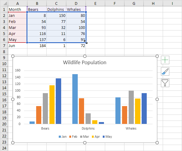
Excel: How to Create a Bubble Chart with Labels - Statology To add labels to the bubble chart, click anywhere on the chart and then click the green plus "+" sign in the top right corner. Then click the arrow next to Data Labels and then click More Options in the dropdown menu: In the panel that appears on the right side of the screen, check the box next to Value From Cells within the Label Options ... A Step-by-Step Guide on How to Make a Graph in Excel Right-click on the chart and click on Add Data Labels to include the values on top of each range. After formatting the histogram accordingly, we arrived at the following graph. This histogram successfully depicts the total number of employees grouped by salary range. This is all you need to know about creating a graph in Excel.

Modifying Axis Scale Labels (Microsoft Excel) Follow these steps: Create your chart as you normally would. Double-click the axis you want to scale. You should see the Format Axis dialog box. (If double-clicking doesn't work, right-click the axis and choose Format Axis from the resulting Context menu.) Make sure the Number tab is displayed. (See Figure 1.)

Add labels to excel graph

How to Add Axis Titles in a Microsoft Excel Chart Select your chart and then head to the Chart Design tab that displays. Click the Add Chart Element drop-down arrow and move your cursor to Axis Titles. In the pop-out menu, select "Primary Horizontal," "Primary Vertical," or both. If you're using Excel on Windows, you can also use the Chart Elements icon on the right of the chart. Format Chart Axis in Excel - Axis Options Analyzing Format Axis Pane. Right-click on the Vertical Axis of this chart and select the "Format Axis" option from the shortcut menu. This will open up the format axis pane at the right of your excel interface. Thereafter, Axis options and Text options are the two sub panes of the format axis pane. How to Add Axis Label to Chart in Excel - Sheetaki Select the chart that you want to add an axis label. Next, head over to the Chart tab. Click on the Axis Titles. Navigate through Primary Horizontal Axis Title > Title Below Axis. An Edit Title dialog box will appear. In this case, we will input "Month" as the horizontal axis label. Next, click OK.

Add labels to excel graph. How to Add Leader Lines in Excel? - GeeksforGeeks Step 2: Go to Insert Tab and select Recommended Charts. A dialogue box name Insert Chart appears. Step 3: Click on All Charts and select Line. Click Ok. Step 4: A line chart is embedded in the worksheet. Step 5: Go to Chart Design Tab and select Add Chart Element . Step 6: Hover on the Data Labels option. Click on More Data Label Options …. excel - How can I add labels with percentage to a pie chart in Python ... It reads an Excel file, checks if there are more locations for one country and if yes, sums the revenues for the locations in the same country and then displays the data as a pie chart using matplotlib. › documents › excelHow to add data labels from different column in an Excel chart? This method will introduce a solution to add all data labels from a different column in an Excel chart at the same time. Please do as follows: 1. Right click the data series in the chart, and select Add Data Labels > Add Data Labels from the context menu to add data labels. 2. › add-vertical-line-excel-chartAdd vertical line to Excel chart: scatter plot, bar and line ... May 15, 2019 · In the modern versions of Excel 2013, Excel 2016 and Excel 2019, you can add a horizontal line to a chart with a few clicks, whether it's an average line, target line, benchmark, baseline or whatever. But there is still no easy way to draw a vertical line in Excel graph. However, "no easy way" does not mean no way at all.

How To Show Two Sets of Data on One Graph in Excel Select the data you want on the graph Once you store the data you want on the graph within the spreadsheet, you can select the data. To do so, click and drag your mouse across all the data you want, including the names of the columns and rows. You can check that you selected the data by looking for the cells to be gray instead of white. 3. › charts › axis-labelsHow to add Axis Labels (X & Y) in Excel & Google Sheets How to Add Axis Labels (X&Y) in Excel. Graphs and charts in Excel are a great way to visualize a dataset in a way that is easy to understand. The user should be able to understand every aspect about what the visualization is trying to show right away. As a result, including labels to the X and Y axis is essential so that the user can see what ... How do I add another label to an Excel chart? Add data labels Click the chart , and then click the Chart Design tab. Click Add Chart Element and select Data Labels, and then select a location for the data label option. Note: The options will differ depending on your chart type. If you want to show your data label inside a text bubble shape, click Data Callout. How to make a quadrant chart using Excel - Basic Excel Tutorial To create it, follow these steps 1. Click on an empty cell 2. Go to the Insert tab 3. On the Charts dialog box, select the X Y (Scatter) to display all types of charts. 5. Click Scatter. An empty chart will appear on your worksheet. Add values to the chart. 1. Right-click on the empty chart area and choose 'Select Data.' 2.

Custom Chart Data Labels In Excel With Formulas Follow the steps below to create the custom data labels. Select the chart label you want to change. In the formula-bar hit = (equals), select the cell reference containing your chart label's data. In this case, the first label is in cell E2. Finally, repeat for all your chart laebls. All About Chart Elements in Excel - Add, Delete, Change - Excel Unlocked The fourth option from the chart element item is for the chart title. On clicking the right arrow, we will find there are three options to change the position of the chart to keep it either above the chart or to overlap it on the chart. More options open the format chart title pane on the left. By default, Excel writes the text string "Chart ... Add labels to numeric axes in a bubble chart - Excel Help Forum Hello - I am trying to add text labels to numeric axes in a bubble chart. I attached a sample workbook that has everything except the labels added. The text I want is shown in the workbook next to the chart. Another question here showed this is possible (I cant post a link, but it ends with: '826640-how-to-change-y-axis-of-bubble-chart-to-non-numeric-values'), but I can't recreate what they did. excel - Formatting Data Labels on a Chart - Stack Overflow Sub ChartTest() ActiveSheet.ChartObjects("Chart 6").Activate z = 1 With ActiveChart If .ChartType = xlLine Then i = .SeriesCollection(1).Points.Count ActiveChart.FullSeriesCollection(1).DataLabels.Select For pts = 1 To i ActiveChart.FullSeriesCollection(1).Points(pts).HasDataLabel = True ' Make sure all points are visible data labels Next pts ...

34 How To Label A Chart In Excel - Label Ideas 2020

How to Make a Pie Chart in Excel & Add Rich Data Labels to The Chart! 7) With the data point still selected, go to Chart Tools>Format>Shape Styles and click on the drop-down arrow next to Shape Effects and select Shadow and choose Inner Shadow>Inside Diagonal Top Left. 8) With the one data point still selected, right-click this data point, and select Add Data Label>Add Data Callout as shown below.

Coordinate Graph Paper Template Axis Labels » ExcelTemplate.net

› Make-a-Bar-Graph-in-ExcelHow to Make a Bar Graph in Excel: 9 Steps (with Pictures) May 02, 2022 · Customize your graph's appearance. Once you decide on a graph format, you can use the "Design" section near the top of the Excel window to select a different template, change the colors used, or change the graph type entirely. The "Design" window only appears when your graph is selected. To select your graph, click it.

Chart's Data Series in Excel - Easy Excel Tutorial

How to Print Labels From Excel - Lifewire Choose Start Mail Merge > Labels . Choose the brand in the Label Vendors box and then choose the product number, which is listed on the label package. You can also select New Label if you want to enter custom label dimensions. Click OK when you are ready to proceed. Connect the Worksheet to the Labels

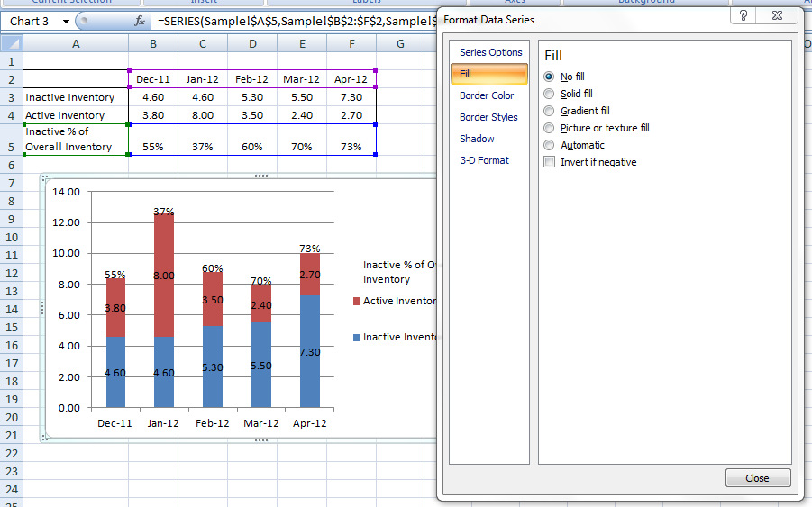
Excel Dashboard Templates How-to Put Percentage Labels on Top of a Stacked Column Chart - Excel ...

How to Apply a Filter to a Chart in Microsoft Excel Select the chart and you'll see buttons display to the right. Click the Chart Filters button (funnel icon). When the filter box opens, select the Values tab at the top. You can then expand and filter by Series, Categories, or both. Simply check the options you want to view on the chart, then click "Apply."

Share :